What you will learn
- What a Kirkwood–Buff integral measures
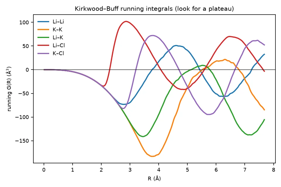
- Why running integrals need a plateau
- Why production work needs large boxes and finite-size corrections
Set up
pip install mace-torch ase matplotlib numpy scipyFiles for this tutorial:
kirkwood_buff.py— Eutectic LiCl–KCl melt, RDFs, running KB integrals../common/models.py— Shared MACE and UMA model loader../common/melt.py— Shared melt builder and structure analysis
Put the shared files in common/, next to the licl-kcl-thermo/ directory. Run the commands from licl-kcl-thermo/.
How it works
Simulate the eutectic melt
58 mol% LiCl with KCl, 64 ion pairs, 800 K, 1.63 g/cm³.
Integrate
Gij(R) = 4π∫₀R(gij(r) − 1) r² dr. A positive G means more j around i than in a random mixture.
Check for a plateau
A trustworthy value needs G(R) to flatten. In a 128-ion box it will not fully flatten. That is the point of this exercise: KB thermodynamics needs big boxes and finite-size corrections such as Krüger et al. (2013).
Run it
The local run used MACE-MP-0 with mace-torch 0.3.17 on an NVIDIA GeForce RTX 5080.
python kirkwood_buff.pyWhat you should see
How this differs from the paper
The in-preparation work uses validated ML potentials, large cells, long runs, finite-size corrections and a composition series to build excess properties and the LiCl–KCl phase diagram. This tutorial shows the method on one small cell.
Full source
kirkwood_buff.py (88 lines)
"""Tutorial — From molten-salt structure to thermodynamics with Kirkwood–Buff integrals.

Kirkwood–Buff (KB) theory links pair structure to thermodynamics. The KB integral
      G_ij = 4π ∫ (g_ij(r) − 1) r² dr
measures how many extra j particles surround an i particle compared with a random mixture.
Combinations of G_ij give activity-coefficient derivatives, partial molar volumes and,
integrated over composition, excess Gibbs energies — and from those a phase diagram.

The in-preparation work does this for molten LiCl–KCl with ML-potential MD. This tutorial runs
one composition and shows the key practical issue: the running integral G(R) must reach a plateau,
and finite boxes make that hard. Production work uses large boxes and finite-size corrections
(e.g. Krüger et al., J. Phys. Chem. Lett. 4, 235 (2013)).

Run:   python kirkwood_buff.py --x-licl 0.58          (eutectic composition; ~5 min on a GPU)
Output: out/kb_running.png, out/rdf_licl_kcl.png
"""
import argparse
import sys
from pathlib import Path

import numpy as np
from ase import units
from ase.md.langevin import Langevin
from ase.md.velocitydistribution import MaxwellBoltzmannDistribution
from ase.optimize import FIRE

sys.path.insert(0, str(Path(__file__).resolve().parents[1] / "common"))
from melt import kb_running, partial_rdf, random_melt  # noqa: E402
from models import get_calc  # noqa: E402

OUT = Path(__file__).parent / "out"
OUT.mkdir(exist_ok=True)


def main():
    ap = argparse.ArgumentParser()
    ap.add_argument("--model", default="mace-small")
    ap.add_argument("--x-licl", type=float, default=0.58)
    ap.add_argument("--n-pairs", type=int, default=64, help="total cation-anion pairs")
    ap.add_argument("--density", type=float, default=1.63, help="g/cm^3, approx. eutectic melt near 800 K")
    ap.add_argument("--T", type=float, default=800)
    ap.add_argument("--steps", type=int, default=6000)
    args = ap.parse_args()

    n_li = round(args.x_licl * args.n_pairs)
    counts = {"Li": n_li, "K": args.n_pairs - n_li, "Cl": args.n_pairs}
    atoms = random_melt(counts, args.density, seed=3, dmin=2.2)
    atoms.calc = get_calc(args.model, dtype="float32")
    FIRE(atoms, logfile=None).run(fmax=0.5, steps=200)
    MaxwellBoltzmannDistribution(atoms, temperature_K=args.T, rng=np.random.default_rng(0))
    dyn = Langevin(atoms, 2.0 * units.fs, temperature_K=args.T, friction=0.01, rng=np.random.default_rng(1))
    frames = []
    for i in range(0, args.steps, 40):
        dyn.run(40)
        if i >= args.steps // 3:
            frames.append(atoms.copy())
        if i % 1000 == 0:
            print(f"step {i:6d}  T = {atoms.get_temperature():6.0f} K", flush=True)

    pairs = [("Li", "Li"), ("K", "K"), ("Li", "K"), ("Li", "Cl"), ("K", "Cl")]
    import matplotlib
    matplotlib.use("Agg")
    import matplotlib.pyplot as plt
    fig1, ax1 = plt.subplots(figsize=(6, 4))
    fig2, ax2 = plt.subplots(figsize=(6, 4))
    for p in pairs:
        r, g = partial_rdf(frames, *p)
        G = kb_running(r, g)
        ax1.plot(r, g, lw=1.8, label=f"{p[0]}–{p[1]}")
        ax2.plot(r, G, lw=1.8, label=f"{p[0]}–{p[1]}")
        tail = G[int(0.75 * len(G)):]
        print(f"G_{p[0]}{p[1]}(R) over last quarter: {tail.mean():8.1f} ± {tail.std():5.1f} Å^3")
    for ax, y in ((ax1, "g(r)"), (ax2, "running G(R) (Å$^3$)")):
        ax.set_xlabel("r (Å)" if ax is ax1 else "R (Å)")
        ax.set_ylabel(y)
        ax.legend(frameon=False, fontsize=8)
    ax2.axhline(0, color="k", lw=0.6)
    ax1.set_title(f"Li$_{{{args.x_licl:.2f}}}$K$_{{{1 - args.x_licl:.2f}}}$Cl melt, {args.T:.0f} K")
    ax2.set_title("Kirkwood–Buff running integrals (look for a plateau)")
    for f, n in ((fig1, "rdf_licl_kcl.png"), (fig2, "kb_running.png")):
        f.tight_layout()
        f.savefig(OUT / n, dpi=160)
    print("wrote", OUT / "kb_running.png")


if __name__ == "__main__":
    main()