What you will learn
- How to build a random melt at a target density
- How to compute partial g(r) and coordination numbers
- What a clustering artifact looks like in g(r)
Set up
pip install mace-torch ase matplotlib numpy scipyFiles for this tutorial:
molten_salt_structure.py— Melt, MD at 1000 K, partial RDFs, Fe–Cl coordination../common/models.py— Shared MACE and UMA model loader../common/melt.py— Shared melt builder and structure analysis
Put the shared files in common/, next to the licl-fecl2-molten/ directory. Run the commands from licl-fecl2-molten/.
How it works
Build the melt
36 LiCl + 12 FeCl₂ (108 ions) are placed randomly in a cubic box at 1.9 g/cm³, with a 2 Å minimum separation. A short FIRE minimization removes close contacts.
Run MD at 1000 K
Langevin dynamics with a 2 fs step. The first third is discarded as equilibration.
Compute g(r)
Partial RDFs for Li–Cl, Fe–Cl, Cl–Cl and Fe–Fe, averaged over frames. The Fe–Cl coordination number is the integral of g(r) up to its first minimum.
Read the Fe–Fe curve
In a well-behaved salt, Cl⁻ separates the Fe²⁺ ions, so Fe–Fe pairs closer than 3 Å are rare. The script counts Fe neighbors within 3 Å of each Fe. A count well above zero, with a sharp Fe–Fe peak near 2.5 Å (the metal bond distance), means the model is clustering Fe. Fine-tuning on DFT data of the melt removed that artifact in the paper.
Run it
The local run used MACE-MP-0 with mace-torch 0.3.17 on an NVIDIA GeForce RTX 5080.
python molten_salt_structure.pyOptional
Install fairchem-core, accept the UMA model terms on Hugging Face, and sign in before running this command.
python molten_salt_structure.py --model uma-s-1p1What you should see
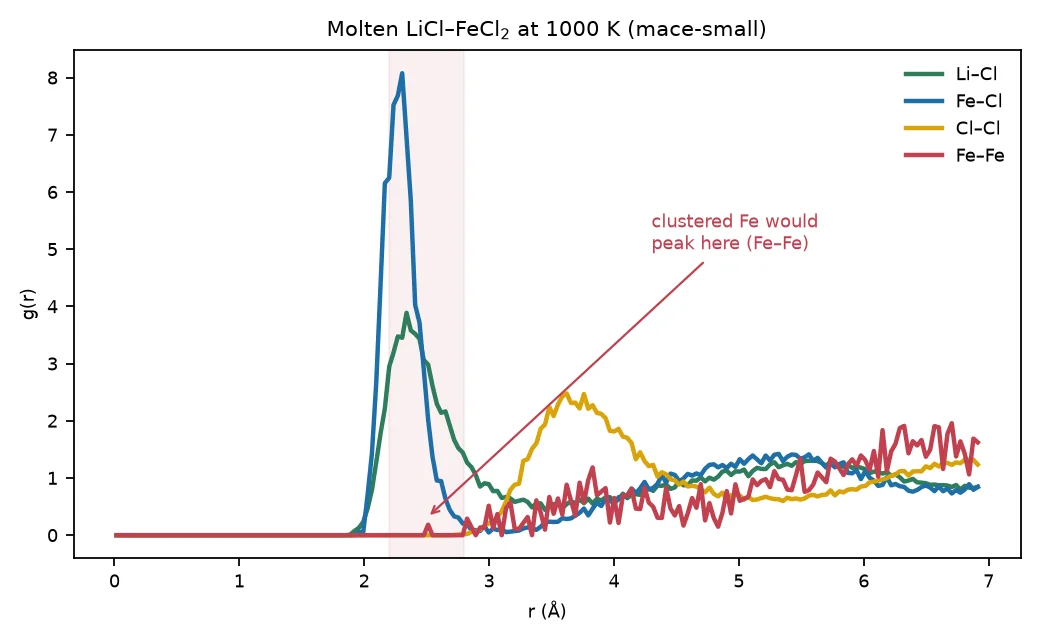
How this differs from the paper
The paper’s models were fine-tuned with multi-head replay and LoRA on DFT data of the melt. They were validated against high-energy X-ray diffraction structure factors (mean R-factor 0.034) over several compositions and temperatures. This tutorial runs only the diagnostic step, with a small cell and short sampling. The fine-tuned models and data will be released with the paper.
Full source
molten_salt_structure.py (99 lines)
"""Tutorial — Check a foundation ML potential on molten LiCl–FeCl2.

The paper (under review) found that universal MACE models, trained mostly on solid crystals,
produce spurious Fe–Fe clustering in molten LiCl–FeCl2. Fine-tuning (multi-head replay + LoRA)
on DFT data of the melt removed the artifact; the fixed model matched high-energy X-ray diffraction.

This tutorial runs the diagnostic you would run first, with the off-the-shelf model:
  1. build a random LiCl–FeCl2 melt at a realistic density
  2. run NVT molecular dynamics at 1000 K
  3. compute partial radial distribution functions g(r) and the Fe–Cl coordination number
  4. inspect Fe–Fe: a sharp first peak near the Fe–Fe metal bond length (~2.5 Å) signals clustering;
     in a well-described salt, Fe ions sit apart, separated by Cl (first Fe–Fe peak near 3.5–4 Å)

Run:   python molten_salt_structure.py                     (~5 min on a GPU; set --steps lower on CPU)
Output: out/rdf.png, out/rdf.csv, out/melt.extxyz
"""
import argparse
import sys
from pathlib import Path

import numpy as np
from ase import units
from ase.io import write
from ase.md.langevin import Langevin
from ase.md.velocitydistribution import MaxwellBoltzmannDistribution
from ase.optimize import FIRE

sys.path.insert(0, str(Path(__file__).resolve().parents[1] / "common"))
from melt import coordination, partial_rdf, random_melt  # noqa: E402
from models import get_calc  # noqa: E402

OUT = Path(__file__).parent / "out"
OUT.mkdir(exist_ok=True)


def main():
    ap = argparse.ArgumentParser()
    ap.add_argument("--model", default="mace-small")
    ap.add_argument("--n-licl", type=int, default=36)
    ap.add_argument("--n-fecl2", type=int, default=12)
    ap.add_argument("--density", type=float, default=1.9, help="g/cm^3 (between molten LiCl ~1.5 and FeCl2 ~2.3)")
    ap.add_argument("--T", type=float, default=1000)
    ap.add_argument("--steps", type=int, default=6000, help="2 fs steps")
    args = ap.parse_args()

    counts = {"Li": args.n_licl, "Fe": args.n_fecl2, "Cl": args.n_licl + 2 * args.n_fecl2}
    atoms = random_melt(counts, args.density, seed=1)
    print(f"{len(atoms)} ions in a {atoms.cell[0, 0]:.2f} Å box")
    atoms.calc = get_calc(args.model, dtype="float32")
    FIRE(atoms, logfile=None).run(fmax=0.5, steps=200)  # remove bad contacts
    MaxwellBoltzmannDistribution(atoms, temperature_K=args.T, rng=np.random.default_rng(0))
    dyn = Langevin(atoms, 2.0 * units.fs, temperature_K=args.T, friction=0.01, rng=np.random.default_rng(1))

    frames = []
    equil = args.steps // 3
    for i in range(0, args.steps, 50):
        dyn.run(50)
        if i >= equil:
            frames.append(atoms.copy())
        if i % 1000 == 0:
            print(f"step {i:6d}  T = {atoms.get_temperature():6.0f} K", flush=True)
    write(OUT / "melt.extxyz", frames)

    pairs = [("Li", "Cl"), ("Fe", "Cl"), ("Cl", "Cl"), ("Fe", "Fe")]
    data = {p: partial_rdf(frames, *p) for p in pairs}
    vol = frames[0].get_volume()
    r, g = data[("Fe", "Cl")]
    rmin = r[np.argmax(g) + np.argmin(g[np.argmax(g):np.argmax(g) + 40])]
    cn = coordination(r, g, counts["Cl"] / vol, rmin)
    rf, gf = data[("Fe", "Fe")]
    n_fefe = coordination(rf, gf, counts["Fe"] / vol, 3.0)  # Fe neighbours closer than 3 Å: the clustering signal
    print(f"Fe–Cl first peak {r[np.argmax(g)]:.2f} Å, coordination {cn:.2f} (cutoff {rmin:.2f} Å)")
    print(f"Fe–Fe neighbours within 3.0 Å: {n_fefe:.2f} per Fe -> "
          f"{'Fe clustering' if n_fefe > 0.5 else 'no clustering: Fe ions stay separated by Cl'}")

    import matplotlib
    matplotlib.use("Agg")
    import matplotlib.pyplot as plt
    fig, ax = plt.subplots(figsize=(6.5, 4))
    col = {("Li", "Cl"): "#2e7d5b", ("Fe", "Cl"): "#1f6fa8", ("Cl", "Cl"): "#d9a20b", ("Fe", "Fe"): "#c2414f"}
    for p, (rr, gg) in data.items():
        ax.plot(rr, gg, lw=2, color=col[p], label=f"{p[0]}–{p[1]}")
    ax.axvspan(2.2, 2.8, color="#c2414f", alpha=0.08)
    ax.annotate("clustered Fe would\npeak here (Fe–Fe)", xy=(2.5, 0.3), xytext=(4.3, 5.0), fontsize=8,
                color="#c2414f", arrowprops=dict(arrowstyle="->", color="#c2414f"))
    ax.set_xlabel("r (Å)")
    ax.set_ylabel("g(r)")
    ax.set_title(f"Molten LiCl–FeCl$_2$ at {args.T:.0f} K ({args.model})")
    ax.legend(frameon=False)
    fig.tight_layout()
    fig.savefig(OUT / "rdf.png", dpi=160)
    np.savetxt(OUT / "rdf.csv", np.column_stack([r] + [data[p][1] for p in pairs]),
               header="r_A " + " ".join(f"g_{a}{b}" for a, b in pairs), fmt="%.4f")
    print("wrote", OUT / "rdf.png")


if __name__ == "__main__":
    main()