What you will learn
- How Lorentz–Berthelot and geometric mixing rules build cross interactions
- Why ion force fields fitted for water can fail at a metal surface
- Where the paper’s rescaling fix enters
Set up
pip install numpy matplotlibFiles for this tutorial:
lj_mixing.py— Au–ion LJ wells for 4 force fields × 2 mixing rules
How it works
Start from the paper’s parameters
Gold uses Heinz et al. (ε = 5.29 kcal/mol, σ = 2.629 Å). Na⁺, Cl⁻ and F⁻ use four published force fields (Jorgensen, Cheatham, Merz, Dang), exactly as listed in Table I.
Mix
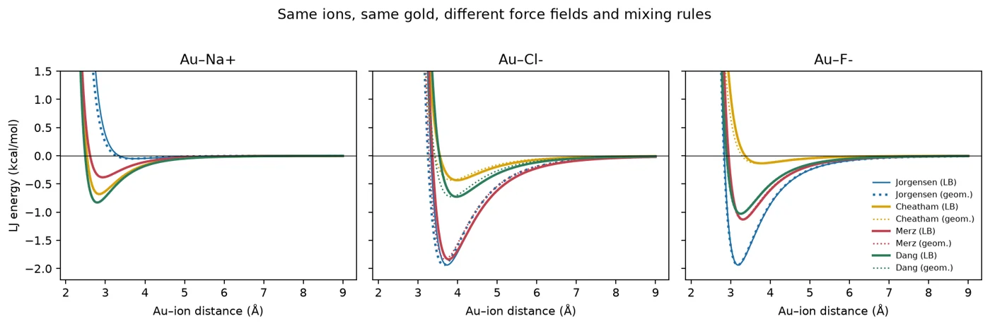
For these force fields, the Au–ion term is built from the pure terms. Both rules use εij = √(εiεj), so they give the same well depth for a given force field. Lorentz–Berthelot averages the size parameter σ arithmetically. Geometric mixing uses √(σiσj). This choice changes the position of the minimum.
Compare the wells
The Au–Cl⁻ well depth ranges from 0.43 to 1.94 kcal/mol across the four force fields. For Na⁺ the range is 0.05 to 0.83 kcal/mol. The spread comes from the force-field parameters. The paper tested how those parameters affect adsorption in water.
Fit to the reference profiles
The authors first varied the gold–sodium well depth. The final fit adjusted both ε and σ to approximate the UMA-S(OMat) free-energy profiles. The classical models still missed specific chloride adsorption.
Run it
python lj_mixing.pyWhat you should see
How this differs from the paper
This reproduces the input to the paper’s analysis, the cross terms. The free-energy profiles themselves come from metadynamics of solvated ions next to a 1,440-atom gold slab in LAMMPS (COLVARS module), plus UMA-based MD. Those runs take days on a cluster.
Full source
lj_mixing.py (95 lines)
"""Tutorial — Why mixing rules can flip the sign of ion adsorption on gold.

Roncoroni, Faiyad et al., J. Chem. Phys. 164, 084702 (2026), Table I lists four popular ion
force fields. Au is modeled with Heinz et al. (2008) parameters. Classical MD never fits the
Au–ion cross term directly: it is built from the pure terms with a mixing rule.

  Lorentz–Berthelot:  sigma_ij = (sigma_i + sigma_j)/2,   eps_ij = sqrt(eps_i eps_j)
  Geometric:          sigma_ij = sqrt(sigma_i sigma_j),    eps_ij = sqrt(eps_i eps_j)

This script computes the Au–ion 12-6 Lennard-Jones well for every force field and both rules.
Well depths vary across force fields. For a given force field, the two mixing rules can shift
the position of the minimum. The paper tested both effects using adsorption free-energy profiles.
The final fit adjusted both eps_ij and sigma_ij to approximate the UMA-S(OMat) profiles.

Run:   python lj_mixing.py            (pure NumPy, < 2 s)
Output: out/au_ion_wells.csv, out/au_ion_lj.png
"""
from pathlib import Path

import numpy as np

OUT = Path(__file__).parent / "out"
OUT.mkdir(exist_ok=True)

AU = (5.29000, 2.6290)  # eps [kcal/mol], sigma [Å]  (Heinz et al. 2008, as used in the paper)
# Table I of the paper: (eps, sigma) for Na+, Cl-, F- and the mixing rule each force field was built with.
FF = {
    "Jorgensen": {"Na+": (0.0005, 4.0700), "Cl-": (0.7100, 4.0200), "F-": (0.7100, 3.0500), "rule": "geometric"},
    "Cheatham":  {"Na+": (0.0874, 2.4393), "Cl-": (0.0356, 4.4777), "F-": (0.0034, 4.1035), "rule": "LB"},
    "Merz":      {"Na+": (0.0276, 2.5996), "Cl-": (0.6380, 4.0981), "F-": (0.2414, 3.2678), "rule": "LB"},
    "Dang":      {"Na+": (0.1300, 2.3500), "Cl-": (0.1000, 4.4500), "F-": (0.2000, 3.1680), "rule": "LB"},
}


def mix(a, b, rule):
    eps = np.sqrt(a[0] * b[0])
    sig = 0.5 * (a[1] + b[1]) if rule == "LB" else np.sqrt(a[1] * b[1])
    return eps, sig


def lj(r, eps, sig):
    x = (sig / r) ** 6
    return 4 * eps * (x * x - x)


rows = []
for ff, d in FF.items():
    for ion in ("Na+", "Cl-", "F-"):
        for rule in ("LB", "geometric"):
            eps, sig = mix(AU, d[ion], rule)
            rows.append((ff, ion, rule, eps, sig, 2 ** (1 / 6) * sig, rule == d["rule"]))

with open(OUT / "au_ion_wells.csv", "w") as f:
    f.write("force_field,ion,mixing_rule,eps_kcal_mol,sigma_A,r_min_A,native_rule\n")
    for r in rows:
        f.write(f"{r[0]},{r[1]},{r[2]},{r[3]:.4f},{r[4]:.4f},{r[5]:.3f},{r[6]}\n")

print(f"{'force field':10s} {'ion':4s} {'rule':9s}  well depth (kcal/mol)  r_min (Å)")
for r in rows:
    print(f"{r[0]:10s} {r[1]:4s} {r[2]:9s}  {r[3]:8.3f}{'  <- native' if r[6] else '':12s}  {r[5]:6.2f}")

# Spread of the native-rule Au–Cl well depth across force fields (the headline of the comparison)
cl = [r[3] for r in rows if r[1] == "Cl-" and r[6]]
print(f"\nAu–Cl- well depth across force fields (native rules): {min(cl):.2f} to {max(cl):.2f} kcal/mol "
      f"({max(cl) / min(cl):.0f}x spread)")

import matplotlib
matplotlib.use("Agg")
import matplotlib.pyplot as plt

r = np.linspace(2.2, 9, 600)
fig, axes = plt.subplots(1, 3, figsize=(12, 3.8), sharey=True)
colors = {"Jorgensen": "#1f6fa8", "Cheatham": "#d9a20b", "Merz": "#c2414f", "Dang": "#2e7d5b"}
for ax, ion in zip(axes, ("Na+", "Cl-", "F-")):
    for ff, d in FF.items():
        for rule, ls in (("LB", "-"), ("geometric", ":")):
            eps, sig = mix(AU, d[ion], rule)
            ax.plot(r, lj(r, eps, sig), ls, color=colors[ff], lw=2 if rule == d["rule"] else 1.2,
                    label=f"{ff} ({'LB' if rule == 'LB' else 'geom.'})")
    ax.axhline(0, color="k", lw=0.6)
    ax.set_ylim(-2.2, 1.5)
    ax.set_xlabel("Au–ion distance (Å)")
    ax.set_title(f"Au–{ion}")
axes[0].set_ylabel("LJ energy (kcal/mol)")
axes[2].legend(fontsize=7, frameon=False, ncol=1, loc="lower right")
fig.suptitle("Same ions, same gold, different force fields and mixing rules", y=1.02)
fig.tight_layout()
fig.savefig(OUT / "au_ion_lj.png", dpi=160, bbox_inches="tight")
print("wrote", OUT / "au_ion_lj.png")


def rescale_eps(eps0, target_scale):
    """Illustrate the paper's initial gold–sodium well-depth sweep at fixed sigma_ij."""
    return eps0 * target_scale